Practical guide

What are you going to learn?

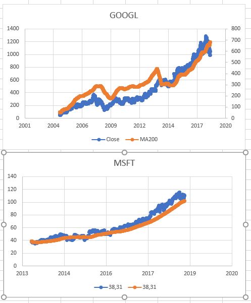
This post explains the solution using stock price data. But you can eventually use Bitcoin data or other cryptocurrency data to do the same calculations. This is a framework for predicting future values regardless of data input.

Trend lines allow us to see the difference in various points over a period of time. This helps to understand the possible path the values might take in the future.

Finding regression line are a very popular tool to illustrate possible outcome and they are used for different business purposes as:

• Demand planning
• Pricing
• Performance
• Risk etc.

You are going to learn about the method, which will help you to calculate the “best fit” line through scatterplots presuming that the only tool you are using is restricted somehow to T-SQL.

To see this trending or for making these “predictions” we will use Microsoft and Google stock prices and hopefully this tutorial would give you enough knowledge to start experimenting with your own business data.

To understand basic principles this short tutorial will walk you through the following:

• Basic elements in math theory about Simple Linear regression.

• Math formula for calculating Linear Regression Coefficients.

• How to write SQL to implement calculation.

• How to test and find right result.

What is Simple Linear Regression and its basic elements?

To get straight to the point – Linear Regression is used to study the relation between two quantitative variables.

We are predicting the value of variable Y named predictor with variable X named response.

If you look through different literature, you will find Predictor and Response can be called differently e.g.

Y – Independent or explanatory variable.

X – Dependent or outcome variable.

Relation between variables

These two variables are related to each other with statistical relationship. This means that variables X and Y are not perfectly correlated to each other.

Just for your information, opposite of statistical relationship is deterministic relationships.

Deterministic relationships

It is the exact relationship between two variables.

For example, the relation between Celsius and Fahrenheit. When the temperature is raising for each Celsius will temperature in Fahrenheit raise for 9/5*Cel+32.  

Statistical relationship

It is opposite from the Deterministic relationship which means that the relationship between the variables is not perfect and change in one variable will result in an increase of another variable, but only approximately.

Math end equation

Linear regression equation

The formula for finding the best-fitting line is y=βx+α where β variable is slope and α is intercept.

Now breaking down formula y=βx+α

What is the Slope?

The slope of a line is a number that describes both the direction and steepness of the line. For example, a slope of 5/2 means that increases on the x-axis by 2 increase the y-value by 5 on average.

What is intercept?

The α – intercept of this line is the value of y at the point where the line crosses the y-axis.

This drawing is showing an example of Scatter Plots, Intercept and Slope.

What is R²

R² is a number between 0 and 1, where 0 indicates that the regression does not represent the data, and 1 is a perfect fit.

If R² is 0,866896156879491, then 86% of the variation can be explained by the regression, and the other 14% of the variation is unexplained. Basically, this says that the model is 86% more accurate than using a random guess (minimum error by using the mean).

We are going to calculate the result for the regression line in simple steps:

• Calculate slope. (Always calculate Slope first because Intercept result is depending on Slope.)

• Calculate intercept.

• Calculate R².

Theoretical stuff stops here and if you want to dive deeper into details, I would recommend reading tons of material on the internet.

I was very glad to read the following:

Solution

Prerequisites

We will create table Historical_Stock_Prices containing for now only Microsoft (MSFT) stock prices.

SQL Code

 CREATE TABLE [dbo].[Historical_Stock_Prices](
            [Dato] [datetime] NULL,
            [Price] [float] NULL
 ) ON [PRIMARY] 

Comments

The code creates an empty table.

Price is “Closing Price”.

Get data from ex. NASDAQ. I have chosen the last 5 years’ stock price data.

Remember to format/change the file so it can be imported into Excel and Copy/Pasted into SQL table afterward.

The second possibility is that to make SSIS package import the file into the table you just created.

SQL Code

Her is SQL code which calculate Slope, Intercept and R²:

 Test of result in Excel

Calculating stock price last 5 years through shown SQL Code are following numbers.

SLOPE	INTERCEPT	R2
0,054647	27,45644236	0,866896

We are going to test this result in Excel:

• Run this query in SQL Management Studio. It will return all rows from Historical_Stock_Prices table.

SELECT

           ROW_NUMBER() over(order by [Dato] asc) as x,

           [Dato],

           Price Amount

FROM [dbo].Historical_Stock_Prices

• Copy data with headers (Right-click on data and then chose “Copy”)
• Paste data in Excel
• Mark data end choose a graph

• Adjust Trendline and set check marks to “Show equation” and “R²” value.
• You should now see the following diagram.

• Numbers marked with yellow (Intercept and Slope) are equal with the result from our SQL code.

Extending of example

Let’s extend our example with the following:

• TREND calculation – can be used in different Reporting tools (Maybe Reporting Services) without statistical features to draw the regression line.

• Additional data – import Google Stock prices into our table together with Microsoft to compare the performance of those two stocks.

For this purpose, we will need to add to our table one extra attribute (Ticker) to distinguish between those two stocks.

Run code below in SQL Management Studio to create missing attribute:

ALTER TABLE dbo.Historical_Stock_Prices ADD Ticker varchar(50) NULL

Next step is to add/update existing and new records with Ticker values.

Run UPDATE and SET “MSFT” value on the new Ticker attribute.

When importing GOOGLE data remember to set “Ticker” with “GOOGL” value.

Extended SQL Code with multiply company stock prices and trend measurements

--drop table #temp
WITH cte AS
(
         SELECT   ticker,
                  Row_number() OVER(partition BY ticker ORDER BY [dato] ASC) AS x,
                  [dato],
                  Sum(price) Amount
         FROM     [PLAYGROUND].[dbo].historical_stock_prices
         GROUP BY ticker,
                  [dato] ), cte1 AS
(
         SELECT   cte.ticker,
                  (Count(x) * Sum(x*amount) – Sum(x) * Sum(amount)) / (Count(x) * Sum(x*x) – Sum(x) * Sum(x))                                        AS SLOPE,
                  Avg(amount)                                                                                                                           AVG_Amount,
                  Avg(x)                                                                                                                                AVG_X,
                  Avg(Cast(amount AS FLOAT)) – ((Count(x) * Sum(x*amount) – Sum(x) * Sum(amount)) / (Count(x) * Sum(x*x) – Sum(x) * Sum(x))* Avg(x)) AS INTERCEPT
         FROM     cte
         GROUP BY cte.ticker )
SELECT     cte.ticker,
           slope,
           avg_amount–(slope*avg_x)                                                                                                                                 AS INTERCEPT,
           (Avg(intercept) * Sum(amount) +Avg(slope) * Sum(x*amount)–Sum(amount)*Sum(amount)/Count(x)) / (Sum(amount*amount) – Sum(amount)* Sum(amount) / Count(x)) AS R2
INTO       #temp
FROM       cte1
INNER JOIN cte
ON         cte.ticker=cte1.ticker
GROUP BY   intercept,
           slope,
           avg_amount,
           avg_x,
           cte.tickerSELECT *
FROM   #tempSELECT   s.ticker,
         Cast(dato AS DATE)                                                                       dato,
         s.price                                                                                  AS amount,
         (Sum(slope)*Row_number() OVER(partition BY s.ticker ORDER BY [Dato] ASC))+Sum(intercept) AS trend
FROM

.Historical_Stock_Prices s  INNER JOIN #temp ON #temp.Ticker=s.Ticker

GROUP by s.Ticker,[Dato], s.Price

Code explanation

• Same explanation as first one just I am grouping on Ticker as well.
  • First CTE is just used to get data from the table.

I am using ROW_NUMBER function to generate numbers that help me calculate X (dependent variable) without converting dates into numbers. 

• Adding Ticker grouping.
  • Second CTE(CTE1) is used to intermediate calculations and to get Intercept and Slope which makes it easier to calculate R² in the final calculation.

• Adding Ticker and TREND calculation. TREND calculation is very useful when showing the Trend line in different Reporting tool and which have no ability to draw a regression line as Excel can.
  • The last calculation (SELECT) is putting everything together. Using Slope and Intercept from CTE1 to calculate R².

As you can see, I am calculating again Intercept just to show that it can be calculated using intermediate variables AVG_Amount and AVG_X from CTE1.

Test of result in Excel with MSFT and GOOGL

Running this SELECT statement (SELECT * FROM #temp) would return following:

Ticker	SLOPE	INTERCEPT	R2
GOOGL	0,260568	-24,56151319	0,830628
MSFT	0,054647	27,45644236	0,866896

#Temp table is generated with SQL code which can be viewed on previous page.

This result is used to compare the result from Excel.

The next picture represents SQL calculated values perfectly matching TREND line (Red) and regression line from Excel (Stipple).  

Conclusion

In this article, we:

• walked through basic linear regression elements
• explored SQL solution regarding Linear Regression
• verified SQL results – explained how to test and compare SQL numbers in Excel.

The result is a small framework for calculating simple linear regression. Just changing data input in SQL code allows calculating a regression for any data

I hope this article would encourage you in the right direction to start the experiment with your own data.